Hyperion Financial Reporting Studio lets you create ranking reports easily by using the built in functionality, but it is available only when there is one dimension on the row. It is also only available for ranking the Top n number of dimensions and not available for the Bottom n number of dimensions. What happens when you want to have more than one dimension on the row or want to rank the Bottom members of a dimension gets more complicated.
 To show the Top 5 products from this list, select row 1 and apply suppression to an row where Column F is > a value of 5. Also, select suppression for where Column F is equal to Zero or No Data. Additionally, using the Grid Properties pane, apply a sort to Row 1 using Column F in ascending order. The column containing the rank can be hidden on the final report.
Using the built in functionality we can create a report of our top 5 products. The product can be put on the row with quarterly and total year Profit on the columns. By highlighting the row, the ability to select the Top n results based upon a column selection becomes available in the Properties pane on the right. The resulting report, shows the top 5 products by year and sorts them in descending order.
There is also a Rank() formula that can be used. This works around both of the drawbacks of the built in Ranking functionality. It allows you to sort ascending or descending. It also allows you to rank members when there is more than one dimension on the row. It will rank based upon the rightmost dimension on the row.
The syntax for the formula is Rank([Reference], Order, Unique(optional)). The Reference can be a cell, row, or column. Order for ascending can be specified as Ascending, Asc, or 1. The order for descending can be specified as Descending, Des, Desc, or 0. Unique is used to indicate how to treat equal values where false gives equal values the same ranking and true gives each value a unique ranking and there is no duplication.
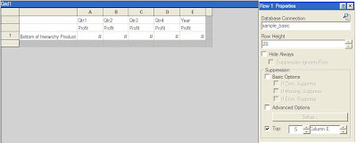
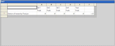
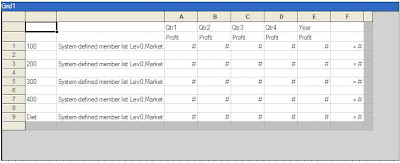
The following achieves the same ranking as above when using the formula Rank([E, 1], Descending ,true). This formula ranks each line but does not filter the results. The ranking for each product can be found in Column F.
To show the Top 5 products from this list, select row 1 and apply suppression to an row where Column F is > a value of 5. Also, select suppression for where Column F is equal to Zero or No Data. Additionally, using the Grid Properties pane, apply a sort to Row 1 using Column F in ascending order. The column containing the rank can be hidden on the final report.Alternatively, a Bottom 5 products report could be created by changing the formula to be Rank([E, 1], Ascending ,true).
Applying all of the same row and report properties as above, here is an example of a report that lists the top 5 markets for each product line.
If there is a need to create a report with both the Top 5 and Bottom 5 members in one report, an additional row can be created for each of the rows. One row will have the rank formula ascending and one will have the formula descending. Additional sorting can be added to the descending rows to have the entire column sorted in order.
An excerpt of the resulting report would be as follows.
 The next hurdle is what happens if there are less than 10 markets with data. This will cause duplication in rows on the report, which is not the desired result.
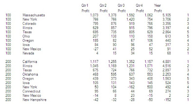
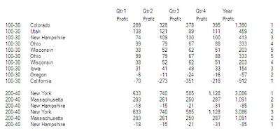 In this example, Ohio and Wisconsin are duplicated for 100-30 since there are only 8 Markets for this product line with data. All 3 markets are duplicated for 200-40, because there are only 3 markets populated.
To work around this duplication issue a Max formula can be used on one of the ranking rows and then suppression can be built on the second that utilizes this Max formula.
In the example, insert a formula row for Row 3. In Column F, specify the formula as Max([2]). Change the Row 2 suppression to exclude the entire row if the Max is less than or equal to 5 and specify to exclude the larger rankings for each of the instances where there between 6 and 9 members in the grouping. The suppression for Row 2 in the sample report would be:
- Data Values in Column F > Value of 5 Or
- Data Values in Column F = Zero Or
- Data Values in Column F = No Data Or
- Value in Cell F,3 <= Value of 5 Or
- ( Value in Cell F, 3 = Value of 6 And
- Data Values in Column F = 5 ) Or
- ( Value in Cell F, 3 = Value of 7 And
- Data Values in Column F = 4 Or
- Data Values in Column F = 5 ) Or
- ( Value in Cell F, 3 = Value of 8 And
- Data Values in Column F = 3 Or
- Data Values in Column F = 4 Or
- Data Values in Column F = 5 ) Or
- ( Value in Cell F, 3 = Value of 9 And
- Data Values in Column F = 2 Or
- Data Values in Column F = 3 Or
- Data Values in Column F = 4 Or
- Data Values in Column F = 5 )
The resulting report will then look exclude the duplications.